Classifier-Free Guidance Explained with a 2-D Diffusion Example

This is a direct follow-up to the earlier 2-D diffusion post. The code below is trimmed to the essentials; the full, runnable version lives in the original notebook: github.com/litlig/notebooks/guided_2d_diffusion.ipynb

What is guided diffusion?

#

In an unguided diffusion model, we sample a noise image and follow the diffusion process to arrive at an image. Often, though, we want to prompt the model to generate a specific kind of image; such generation is called guided generation.

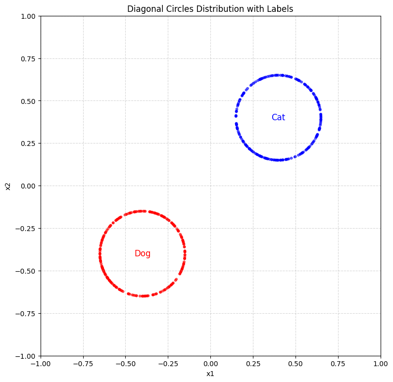
We continue with the 2-dimensional example — a two-pixel image. We say the cluster in the upper right are cat images, and the cluster in the lower left are dog images.

Vanilla guidance

#

With a text label/prompt \(y\), we want to learn a guided vector field that moves the probability mass toward the distribution of images conditioned on the label, \(p_{data}(\cdot\,|\,y)\).

Intuitively, we can follow the same procedure as unguided flow matching. For each training example, we sample a pair of image and label (or text caption). We train a neural network to estimate the conditional vector field, giving it the label \(y\) as an additional input. The loss function is still the mean squared error:

When the target \(z\) is given, the conditional vector field is computed the same way as before:

The label enters the network through an embedding, which is concatenated with \(x_t\) and \(t\):

class ConditionalFlowModel(nn.Module):
  def __init__(self, embedding_dim=2, num_classes=2):
    super().__init__()
    self.embedding = nn.Embedding(num_classes, embedding_dim)
    input_size = 2 + 1 + embedding_dim  # xt + t + label embedding
    self.net = nn.Sequential(
        nn.Linear(input_size, 128), nn.SiLU(),
        nn.Linear(128, 128), nn.SiLU(),
        nn.Linear(128, 128), nn.SiLU(),
        nn.Linear(128, 2),
    )

  def forward(self, xt, t, y):
    y_embedded = self.embedding(y.squeeze(-1))
    return self.net(torch.cat([xt, t, y_embedded], dim=-1))

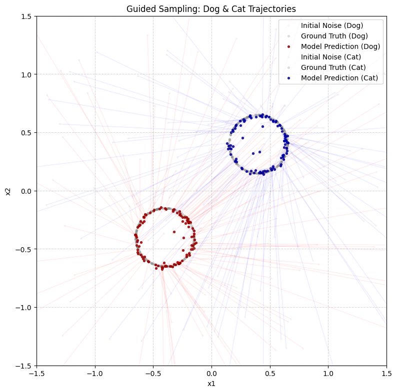
Sampling then just fixes the guidance label and integrates the field with Euler steps. With guide_label=0 we pull noise toward the dogs, with guide_label=1 toward the cats:

Classifier-free guidance

#

In this simple example, the vanilla approach above already works reasonably well. In practice, though, samples from such a model often don’t follow the prompt or label very strongly. The guided probability path is \(p_t(x\,|\,y)\). By Bayes’ theorem:

Taking the log of both sides and then the gradient with respect to \(x\) (the \(p_t(y)\) term drops out, since it doesn’t depend on \(x\)):

\(\nabla \log\) is the score function. For a Gaussian probability path, the vector field relates to the score by \(v_t(x) = \alpha_t \nabla \log p_t(x) + \beta_t x_t\). Substituting gives a formula that connects the two vector fields:

The extra term \(\nabla \log p_t(y\,|\,x)\) is what contributes the guidance. A natural way to make generation follow the guidance more strongly is to scale this term up. Estimating \(p_t(y\,|\,x)\) is essentially a classification problem — given a noisy sample \(x\), predict its label — so this approach is called classifier guidance (Dhariwal & Nichol, 2021): it requires training one network for the vector field and a separate classifier.

A more elegant approach, classifier-free guidance (Ho & Salimans, 2022), eliminates the need for a separate classifier. Given the guided vector field \(v_t(x\,|\,y)\) and the unguided vector field \(v_t(x)\), the influence of guidance is \(v_t(x\,|\,y) - v_t(x)\). We scale it up by a weight \(w > 1\) and use the following in forward sampling:

\(w\) is called the guidance scale. Rearranged, this is the form you will usually see in papers and code, written for a noise-prediction model \(\epsilon_\theta\):

It is the same combination: the unconditional prediction plus \(w\) times the guidance direction.

To get both \(v_t(x)\) and \(v_t(x\,|\,y)\) from a single network, we treat the unguided vector field as a guided one with a special null prompt, which we inject at random into a fraction of the training samples. This trick is usually called label dropout (or conditioning dropout); dropping 10–20% of labels is typical, so the same network learns both fields:

def get_batch(dist_fn, batch_size, inject_rate=0.1):
  z, y = dist_fn(batch_size)
  z = torch.from_numpy(z).float()
  y = torch.from_numpy(y).long().unsqueeze(1)
  x0 = torch.randn(batch_size, 2)
  t = torch.rand(batch_size, 1)
  xt = (1 - t) * x0 + t * z
  vf = z - x0

  # Randomly replace some labels with the special 'null' label (2)
  num_inject = int(batch_size * inject_rate)
  if num_inject > 0:
    inject_indices = torch.randperm(batch_size)[:num_inject]
    y[inject_indices] = 2
  return xt, t, y, vf

At sampling time we run the network twice per step — once with the real label, once with the null label — and combine them with the guidance weight:

def cfg_sample(model, nsample, steps=100, guide_label=0, weight=2.0):
  null_label = 2
  x = torch.randn(nsample, 2)
  dt = 1.0 / steps
  y_guide = torch.full((nsample, 1), guide_label, dtype=torch.long)
  y_null  = torch.full((nsample, 1), null_label,  dtype=torch.long)
  for step in range(steps):
    t = (step / steps) * torch.ones(nsample, 1)
    vf_guided   = model(x, t, y_guide)
    vf_unguided = model(x, t, y_null)
    x = x + ((1 - weight) * vf_unguided + weight * vf_guided) * dt
  return x

Sweeping the guidance weight shows its effect directly. At \(w=1\) we recover plain conditional sampling. As \(w\) grows, the guidance term is amplified: samples cling more tightly to their target cluster and drift further from the opposite one — the samples follow the prompt more faithfully, at the cost of some diversity as they concentrate.

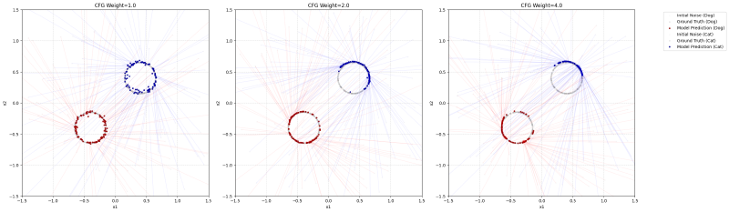
In image models the guidance scale is usually set well above 1; Stable Diffusion defaults to 7.5. Push it too high and samples become oversaturated and repetitive, the same fidelity-versus-diversity trade-off visible in the 2-D plot.

Classifier guidance vs classifier-free guidance

#

• Classifier guidance trains a separate classifier on noisy samples \(x_t\) at every noise level and adds its gradient during sampling. It can steer an existing unconditional model, but the classifier has to cope with heavy noise, and following its gradient risks pushing samples toward whatever fools the classifier rather than toward better samples.
• Classifier-free guidance needs only one network trained with label dropout, at the cost of two forward passes per sampling step. It works with any conditioning that can be dropped (class labels, text prompts, images), which is why text-to-image models like Stable Diffusion use it.